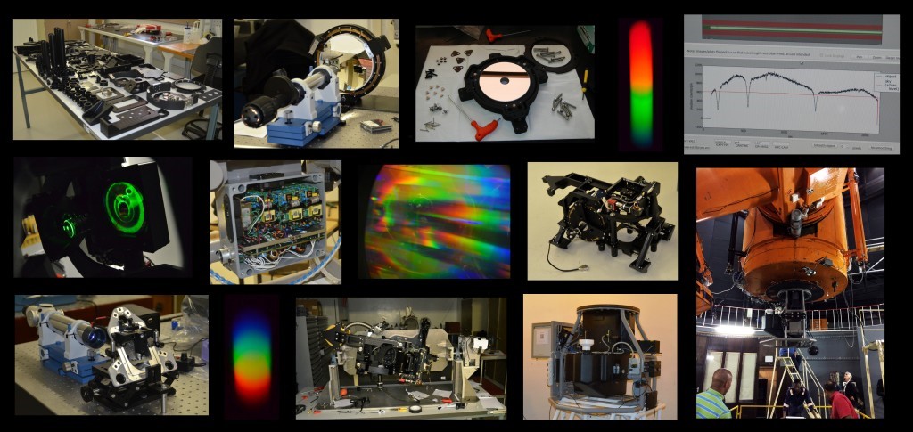
The Cassegrain Spectrograph Upgrade project was completed in October 2015 and the instrument (SpUpNIC) has been in routine operation and well subscribed ever since. A SpUpNIC paper was presented at the SPIE Astronomical Telescopes and Instrumentation conference in Edinburgh in June 2016.
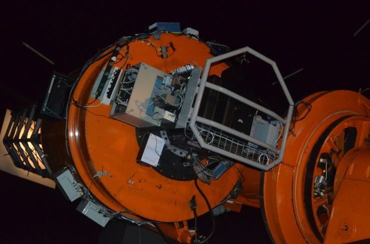
SpUpNIC still uses the same set of surface-relief diffraction gratings, arc lamps (CuAr and CuNe – now available simultaneously) and order blocking filters (BG38, BG39 and GG495) as before, but the instrument has new camera and collimator optics, as well as a new detector system. The new optics and CCD slightly reduce the dispersion, but significantly increase the wavelength ranges delivered by the various gratings – see the table below for details. The original slit mechanism is still in use and offers slit widths ranging from 0.15″ to 4.2″ (in 0.15″ increments).
| GRATING | LINES PER MM |
BLAZE (Å) |
RANGE (Å) |
DISPERSION (Å/PIXEL) |
ARC MAP |
| 4 | 1200 | 4600 | 1250 | 0.625 | 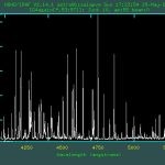 |
| 5 | 1200 | 6800 | 1100 | 0.525 |  |
| 6 | 600 | 4600 | 2800 | 1.36 |  |
| 7 | 300 | 4600 | 5550 | 2.72 | 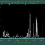 |
| 8 | 400 | 7800 | 4100 | 2.21 | 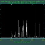 |
| 9 | 830 | 7800 | 1700 | 0.830 | 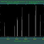 |
| 10 | 1200 | 10000 | 950 | 0.470 | 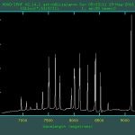 |
| 11 | 600 | 10000 | 2600 | 1.25 | 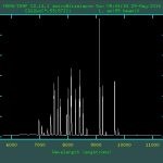 |
| 12 | 300 | 10000 | 5600 | 2.75 | |
The spectrograph camera’s new Folded-Schmidt optical design is much more efficient than the old Maksutov-Cassegrain system, and the new CCD provides an additional sensitivity boost. The introduction of a rear-of-slit viewing camera allows far more accurate positioning of the target on the slit, and being able to view the star going down the slit makes it easier to focus the telescope reliably. These critical aspects have substantially increased the spectrograph throughput and overall observing efficiency, particularly for faint targets. The new instrument control software, as well as the quick-look data reduction tool, further streamline the process and provide access to the data which can be extracted and approximately wavelength calibrated as soon as an image is read out.
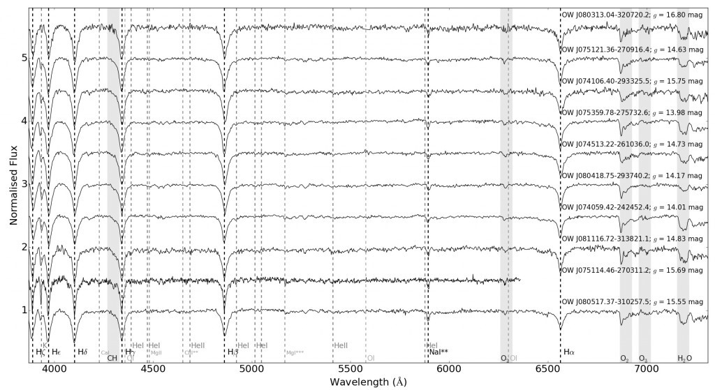
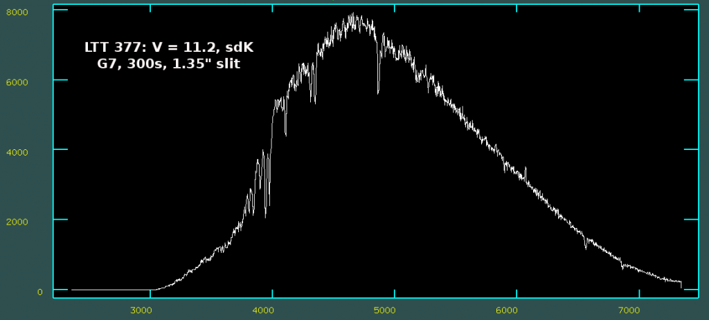
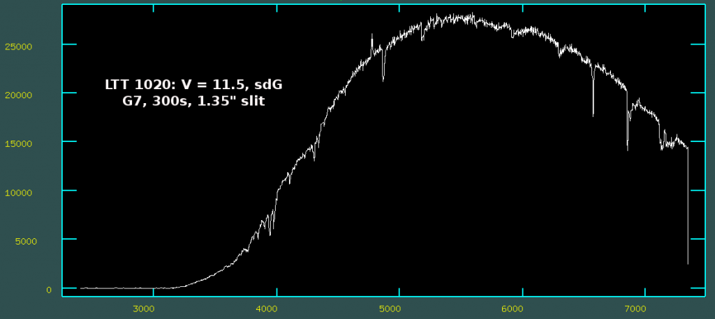
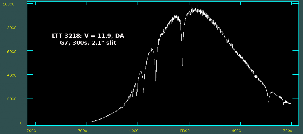
Sample spectra are shown in the figure below, with the SDSS g magnitudes of the stars listed to the right. Most were obtained with the low resolution G7, but the shorter spectrum (second from the bottom) was a 900s exposure with a 1.5″ slit using G6. The G7 spectra employed slit widths between 1.5″ and 2.7″ (depending on the seeing) and the exposure times ranged between 1800 sec for 16-18 mag, 1200 sec for 15-16 mag, 600-900 sec for 13-15 mag and 200 sec for 11th/12th mag standard stars. The faintest target observed for this campaign was 18th mag and that required a 2400 sec exposure. The most extreme use of the high resolution blue G4 has been to observe a V~17.5 mag star for 1200 sec and be able to classify the object as a white dwarf.
Spectro-photometric Standards with Grating 4
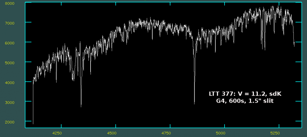
Spectro-photometric Standards with Grating 5
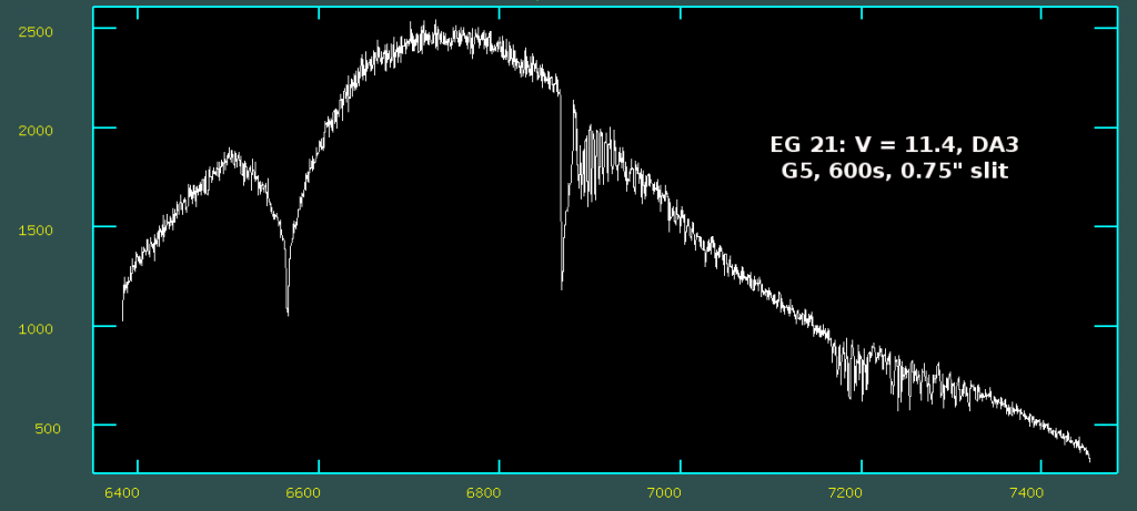
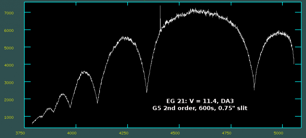
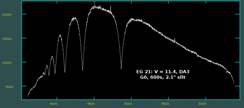
Spectro-photometric Standards with Grating 6
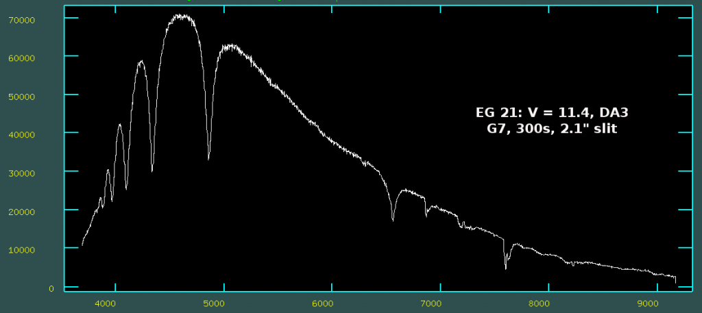
Spectro-photometric Standards with Grating 7
The instrument team is completing remaining commissioning tasks and tests, and making refinements to the system – specifically the software, as well as the grating mechanism which proved to be mechanically unstable. The latter has been significantly improved and ought to be resolved with the modifications currently in progress. As a result, we do not yet have a good feel for the instrument’s performance in terms of measuring radial velocities. This information will be added once the grating stability issues have been addressed and the RV capabilities of the instrument can be established.
The SpUpNIC Wiki page provides detailed information for observers at the telescope, start-offs are provided for new users and telephonic support is available throughout the night should problems arise at the telescope.
SpUpNIC Exposure Time Information
For users wishing to estimate exposure times from real SpUpNIC data, the following files give extracted 1D spectra from a representative subset of a suite of spectrophotometric standards observed with SpUpNIC during 2015 Nov-Dec. The most reliable way to estimate exposure times is probably to measure S/N directly in the wavelength range of interest, with the setup which most closely matches yours, and then to scale accordingly.
Measurements are given for the two most commonly used gratings, G4 and G7, and at typical grating angles. These conversion factors should be approximately unchanged for small changes in grating angle. Other gratings will be added as the information becomes available.
Each _1D.txt file contains wavelength (A) and [sky subtracted] counts summed over the extraction window in the spatial direction. This is the raw counts observed in the total exposure time. Exposure times and other useful info are given in the NOTES file. These files are the output from V2 (May 2016) of the quick look GUI and include automatic wavelength calibration. These are not yet finely tuned, but should be accurate to better than ~2A, and thus fine for comparing with flux standards.
Also included are files containing the conversion factors to convert from **counts/second/pixel** into flux units in 10^-16 erg/s/cm^2/A. So, in order to go from the observed counts in the _1D.txt files, it is necessary to divide by the exposure time and then multiply by the appropriate conversion factor.
All of these observations were made in “Faint & Slow” mode, which has a gain of 1.145e-/ADU. No aperture correction has been made.
| Filename | Grating | Grating Angle | Object | EXPTIME | Comments |
| a0053955_1D | G4 | 4.1 | LTT_377 | 600 | 2.1″ slit in 1.5″ seeing |
| a0071045_1D | G7 | 17.0 | LTT_377 | 300 | 1.35″ slit in ? seeing |
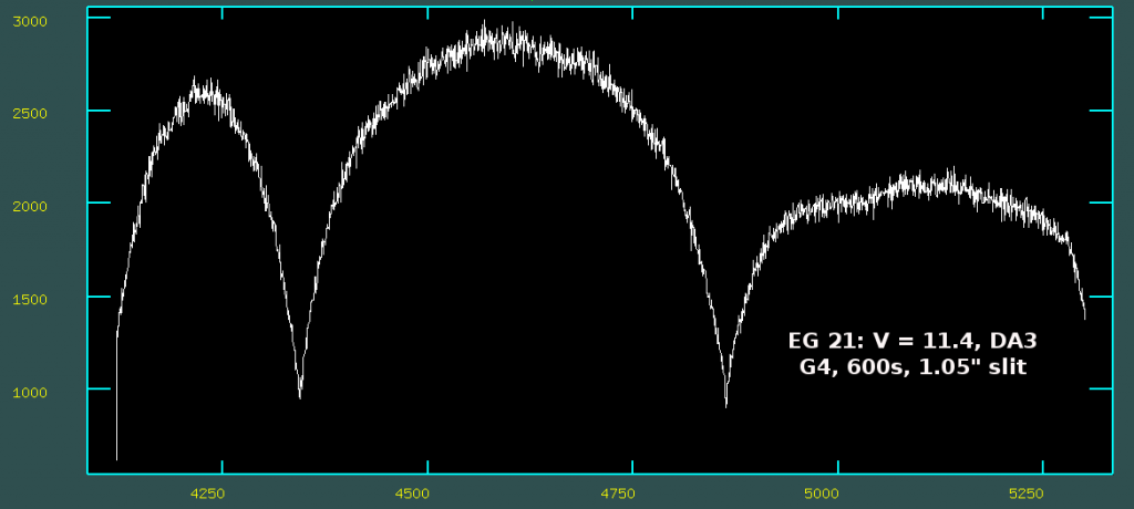
| a0071110_1D | G7 | 15.3 | EG21 | 300 | 2.1″ slit in 1.2″ seeing |
A more detailed version of this table: NOTES
The observed S/N may be simply estimated in the wavelength range of interest by, for example in python:
x,y = np.loadtxt(‘a0071110_1D.txt’,unpack=True, usecols=(0,1)) # read in data
ok = np.where( (x>5100.) & (x<5200.) )[0] # choose wavelength range relatively free of absorption lines
print median(y[ok])/std(y[ok])
76.043849269
Therefore, for LTT 377 at ~5150A (flux ~1.2e-13 erg/s/cm^2/A) SpUpNIC reaches a S/N ~76 PER CCD PIXEL in 600s.
Flux calibration curves
gr7_calfac_grang17.0
gr7_calfac_grang15.3
gr4_calfac_grang4.1
The Hamuy standards used in the calibration can be found here:
ftp://ftp.eso.org/pub/stecf/standards/ctiostan/ NOTE: LTT377 is cd_34d241
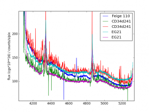
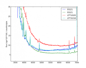
Approximate polynomial fits to a series of standard stars, giving the factor by which to multiply the raw counts (per second), to get to flux, as described above. The plots below show the stars used (and the variation from object-to-object) for G4 and G7 respectively. Note: LTT1020 seems to be an outlier and has been rejected from the fits. It may be necessary to interpolate the wavelengths onto a common grid before multiplying.
Quick Python Example:
x,y = np.loadtxt(‘a0071110_1D.txt’,unpack=True, usecols=(0,1)) # read in data
y = y / 600. # convert to counts/s
a,b = np.loadtxt(‘gr7_calfac_grang15.3.txt’,unpack=True, usecols=(0,1)) # read in appropriate flux conversion factor
# interpolate to same wavelength bins:
ib = np.interpol(x,a,b)
plot(x, y*ib*1e-16 ) # flux calibrated in erg/s/cm^2/A
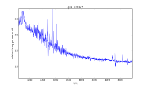
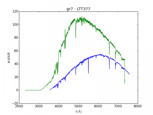
Comparison with Pre-Upgrade Spectrograph
For users preferring to scale their exposure times from previous experience, the following may be more useful.
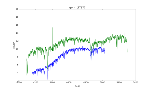
G4
Comparison of pre-upgrade (blue) vs SpUpNIC (green) in e-s per second **per A**. Note: the dispersion has changed from 0.495 A/pix to 0.622 A/pix and this conversion factor has been included. The old gain was 1e-/ADU. To compare values per CCD pixel, SpUpNIC will be 0.622/0.495 times higher than plotted. To compare old and new counts, SpUpNIC will be 1.145 times lower (the new gain).
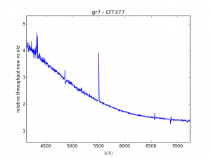
Relative throughput (ratio of the above). Not smoothed.
As above, but for G7.
SpUpNIC Instrument Team
SpUpNIC was an effort undertaken by a large team of people, over a very long period of time. The PI on the project was Lisa Crause (aka the fearless leader).
We encourage proper credit be given to the instrument teams, which means that co-authorship for the following groups would be appreciated for publications stemming from data taken during commissioning time. This follows the standard instrument commissioning agreement for SpUpNIC.
Full Instrument Team
L.A. Crause, D.B. Carter, A. Daniels, G.P. Evans, P. Fourie, D. G. Gilbank, M. Hendricks, W. Koorts, D. Lategan, E. Loubser, S. Mouries, J. O’Connor, D. O’Donoghue, S.B. Potter, C. Sass, A.A. Sickafoose, J. Stoffels, P. Swanevelder, C. van Gend, M. Visser, H.L. Worters
The full team includes all staff who have made a significant contribution to the project. Notably, this includes workshop staff and technicians (non-scientists).
Typically, the instrument PI is the lead author on the papers and publications in which the instrument is described. Regardless of the first author, the full instrumentation team should be provided the opportunity to be coauthors on the first instrument presentation (e.g. at an SPIE meeting) and on the instrument publication. The decision to be a co-author rests with each individual, such that they can opt out if desired.
Instrument Science Team
L.A. Crause, D. G. Gilbank, D. O’Donoghue, S.B. Potter, A.A. Sickafoose, C. van Gend, H.L. Worters
The science team consists of PhD-level staff who have contributed significant time and/or effort to the construction of the instrument. This is a subset of the full instrument team.
Users of an instrument while it is undergoing commissioning are strongly encouraged to credit the instrument science team in all publications stemming from data taken during that time. Without these people, the instrument would not be available!