Instruments List by telescope
1.9-m Telescope
SpUpNIC – Long-slit spectrograph
SHOC – High-speed imaging camera
HIPPO – High-speed photo-polarimeter
1.0-m Telescope
SAAO CCD Camera (STE3/STE4) – Imaging cameras
SHOC – High-speed imaging camera
Lesedi
SHOC – High-speed imaging camera
Sibonise – Wide-field imaging camera
Mookodi – Low-resolution slit-spectrograph & imager
Instrumentation Electronics
The Electronics department of the Instrumentation Division is responsible for developing, maintaining and supporting the electronic components of the telescopes and instruments.
Team members include Hitesh Gajjar (head of department), Piet Fourie, Willie Koorts, Pieter Swanevelder, Michael Rust, Avhapfani Malaudzi, Reggie Klein and Keegan Titus.
Software Framework
We have developed a new software framework which we intend using for all new and upgraded instruments on the SAAO small and medium telescopes. The framework is distributed, in that it allows components to exist independently yet communicate through a network, and language-agnostic, in that it allows components to be written in whichever language is most suitable to the task at hand.
At its core is the Apache Thrift package. This allows interfaces to be defined in a straightforward way, and then generates boiler-plate code to implement the interface. Thrift provides both a means of interprocess communication and remote procedure calls.
The framework allows the user interface to be separate and remote from the back-end code. We are using this framework to develop web-based interfaces, so that in future users will not neccessarily need to be at the telescope to operate the instruments.
The framework has been applied to the Sutherland High-speed Optical Camera (SHOC) systems, where the user is now able to interact with the filter wheel, global positioning system (GPS) and camera through a single (web-based) interface. We installed the revamped SHOC systems in early 2015. We also used the framework to develop software for the upgraded Cassegrain spectrograph on the 74-inch telescope, which went live in October 2015.
Instruments We’re Building
We are continuously upgrading and improving our instruments, and we’ve always got several things on the go. Our highest priority project at the moment is Sibonise, a wide-field camera to be mounted on one of the Nasmyth ports of Lesedi (the SAAO’s new 1-metre telescope). This will incorporate the largest detector ever handled by our instrumentation team (6k x 6k pixels!) and we are using the IDSAC controller developed by the Indian Inter-University Centre for Astronomy and Astrophysics (IUCAA). The cryostat, instrument housing, filter and shutter mechanisms have all been designed and are being built-in-house, in out mechanical and electronics workshops. The software is being developed using the software framework previously developed and used for the SHOC and SpUpNIC instruments.
We have developed a new software framework which we are now using for all new and upgraded instrumentation projects. The framework supports a distributed set of instrument components, and allows a web-based user interface to be implemented. This is in line with our long-term goal of having the instruments be remotely (and eventually robotically) operable.
The software for the SHOC instruments has been re-written using the new framework, and went live in the second quarter of 2015. As part of the rewrite, a web interface to the instrument is provided, and all the hardware components (camera, GPS and filter wheel) are controlled from a single interface. This also allows the generated FITS data files to be populated with information from all components.
In addition to the instruments, we are also developing new control systems for the telescopes. The Telescope Control System integrates all the different functions of the telescope such as telescope movement, dome and shutter control and any other parts of the telescope that requires control. We are working towards full remote control of the telescope and telescope environment. Safety features are incorporated in the designs to ensure that the telescope or users are protected in the events such as power failures, bad weather conditions and moving of the telescope or dome where things can be damaged. Some of these features that we have developed for telescopes and environment are incorporated by some of the other facilities we host at SAAO.
We proudly utilize the following software in the design and development of our instruments:


SpUpNIC: Spectrograph Upgrade – Newly Improved Cassegrain
The Cassegrain Spectrograph Upgrade project was completed in October 2015 and the instrument (SpUpNIC) has been in routine operation and well subscribed ever since. A SpUpNIC paper was presented at the SPIE Astronomical Telescopes and Instrumentation conference in Edinburgh in June 2016.
SpUpNIC still uses the same set of surface-relief diffraction gratings, arc lamps (CuAr and CuNe – now available simultaneously) and order blocking filters (BG38, BG39 and GG495) as before, but the instrument has new camera and collimator optics, as well as a new detector system. The new optics and CCD slightly reduce the dispersion, but significantly increase the wavelength ranges delivered by the various gratings – see the table below for details. The original slit mechanism is still in use and offers slit widths ranging from 0.15″ to 4.2″ (in 0.15″ increments).
| GRATING | LINES PER MM |
BLAZE (Å) |
RANGE (Å) |
DISPERSION (Å/PIXEL) |
ARC MAP |
| 4 | 1200 | 4600 | 1250 | 0.625 |  |
| 5 | 1200 | 6800 | 1100 | 0.525 |  |
| 6 | 600 | 4600 | 2800 | 1.36 | 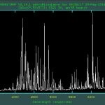 |
| 7 | 300 | 4600 | 5550 | 2.72 | 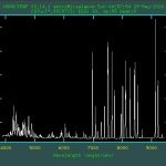 |
| 8 | 400 | 7800 | 4100 | 2.21 | 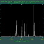 |
| 9 | 830 | 7800 | 1700 | 0.830 | 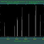 |
| 10 | 1200 | 10000 | 950 | 0.470 | 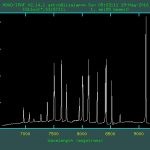 |
| 11 | 600 | 10000 | 2600 | 1.25 | 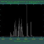 |
| 12 | 300 | 10000 | 5600 | 2.75 | |
The spectrograph camera’s new Folded-Schmidt optical design is much more efficient than the old Maksutov-Cassegrain system, and the new CCD provides an additional sensitivity boost. The introduction of a rear-of-slit viewing camera allows far more accurate positioning of the target on the slit, and being able to view the star going down the slit makes it easier to focus the telescope reliably. These critical aspects have substantially increased the spectrograph throughput and overall observing efficiency, particularly for faint targets. The new instrument control software, as well as the quick-look data reduction tool, further streamline the process and provide access to the data which can be extracted and approximately wavelength calibrated as soon as an image is read out.
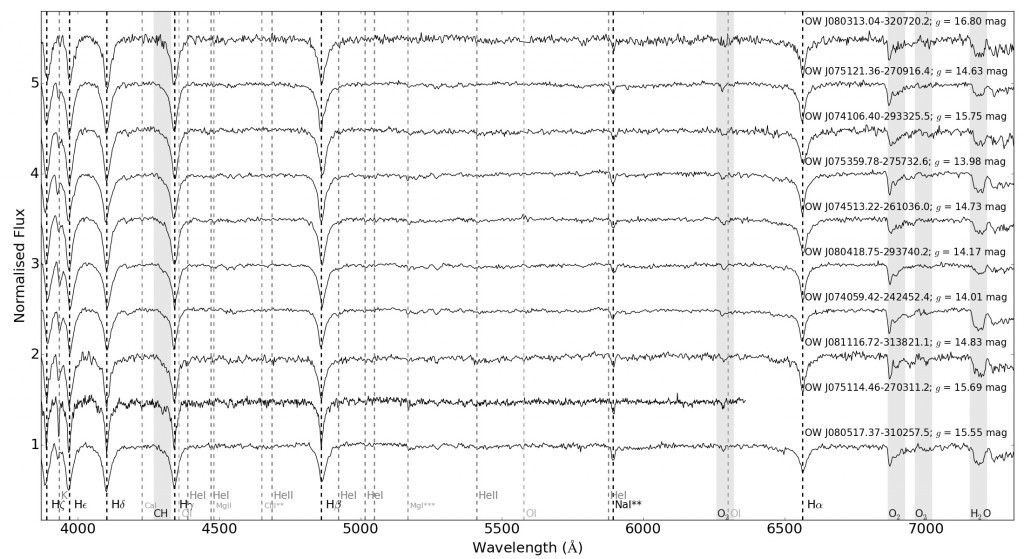
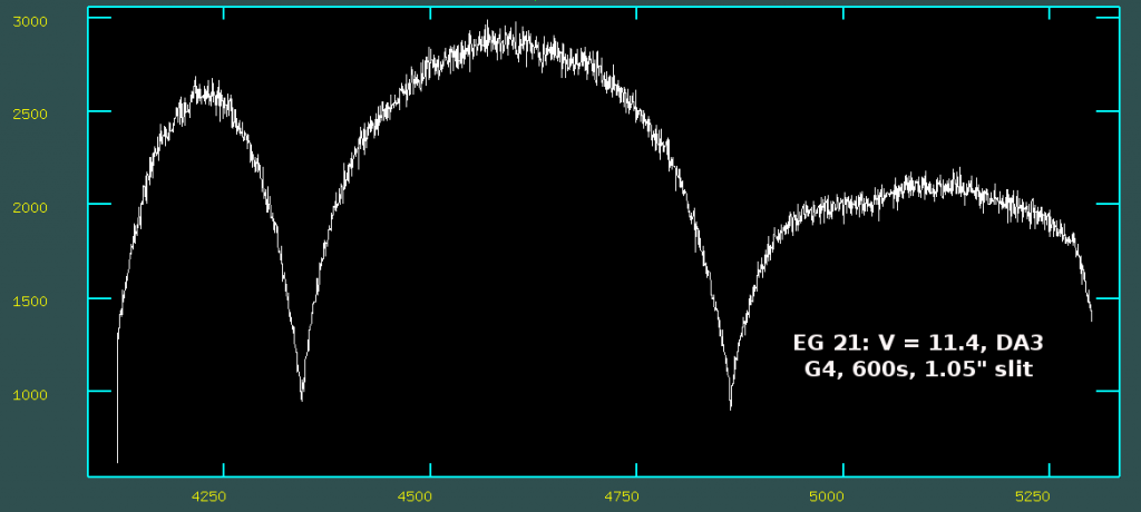
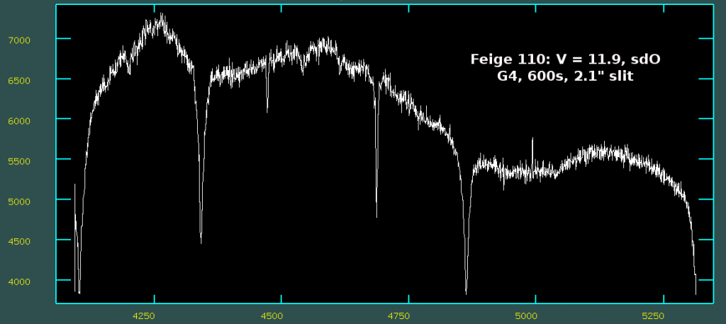
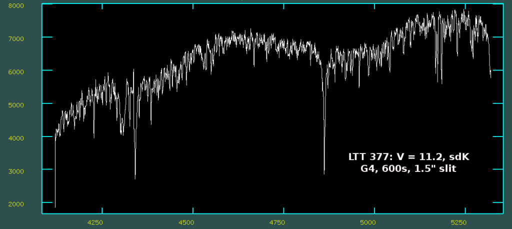
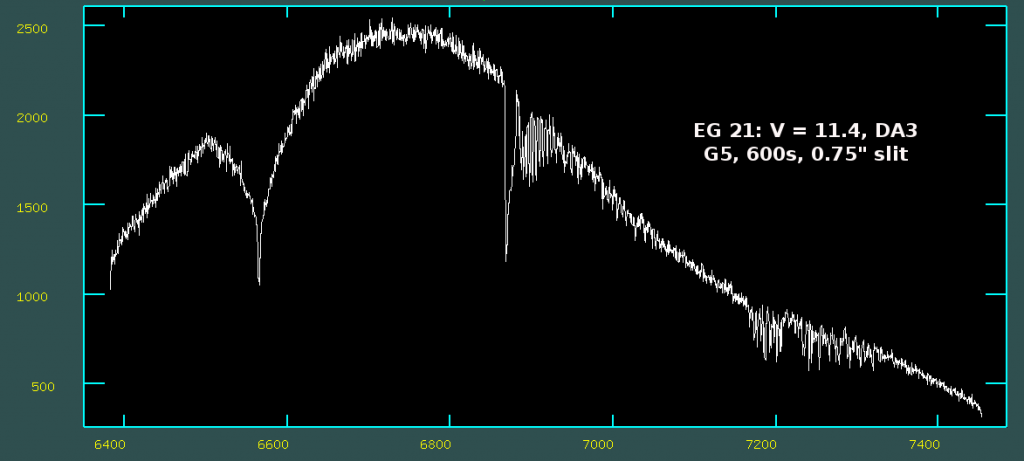
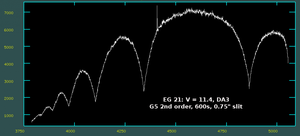
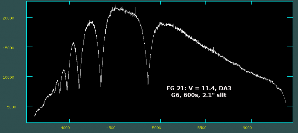
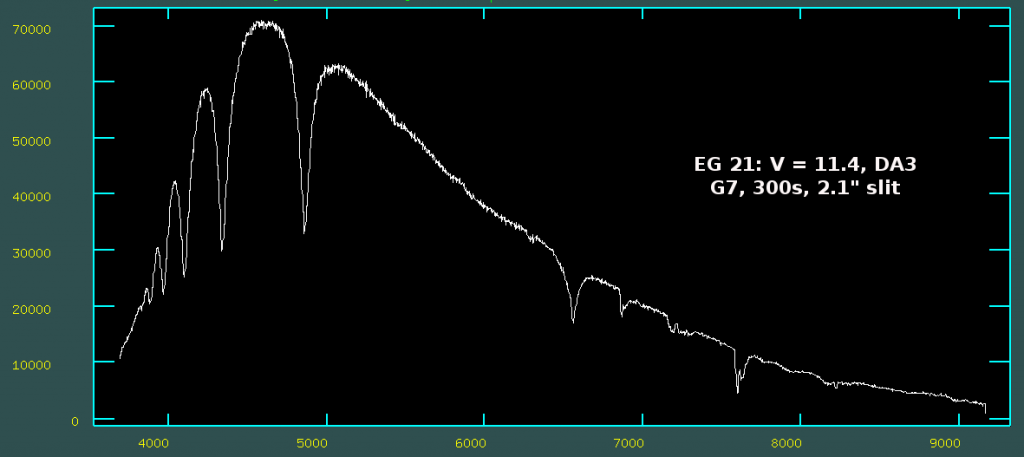
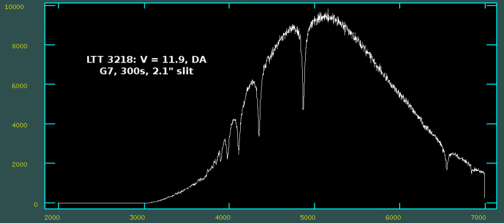
Sample spectra are shown in the figure below, with the SDSS g magnitudes of the stars listed to the right. Most were obtained with the low resolution G7, but the shorter spectrum (second from the bottom) was a 900s exposure with a 1.5″ slit using G6. The G7 spectra employed slit widths between 1.5″ and 2.7″ (depending on the seeing) and the exposure times ranged between 1800 sec for 16-18 mag, 1200 sec for 15-16 mag, 600-900 sec for 13-15 mag and 200 sec for 11th/12th mag standard stars. The faintest target observed for this campaign was 18th mag and that required a 2400 sec exposure. The most extreme use of the high resolution blue G4 has been to observe a V~17.5 mag star for 1200 sec and be able to classify the object as a white dwarf.
Spectro-photometric Standards with Grating 4
Spectro-photometric Standards with Grating 5
Spectro-photometric Standards with Grating 6
Spectro-photometric Standards with Grating 7
The instrument team is completing remaining commissioning tasks and tests, and making refinements to the system – specifically the software, as well as the grating mechanism which proved to be mechanically unstable. The latter has been significantly improved and ought to be resolved with the modifications currently in progress. As a result, we do not yet have a good feel for the instrument’s performance in terms of measuring radial velocities. This information will be added once the grating stability issues have been addressed and the RV capabilities of the instrument can be established.
The SpUpNIC Wiki page provides detailed information for observers at the telescope, start-offs are provided for new users and telephonic support is available throughout the night should problems arise at the telescope.
SpUpNIC Exposure Time Information
For users wishing to estimate exposure times from real SpUpNIC data, the following files give extracted 1D spectra from a representative subset of a suite of spectrophotometric standards observed with SpUpNIC during 2015 Nov-Dec. The most reliable way to estimate exposure times is probably to measure S/N directly in the wavelength range of interest, with the setup which most closely matches yours, and then to scale accordingly.
Measurements are given for the two most commonly used gratings, G4 and G7, and at typical grating angles. These conversion factors should be approximately unchanged for small changes in grating angle. Other gratings will be added as the information becomes available.
Each _1D.txt file contains wavelength (A) and [sky subtracted] counts summed over the extraction window in the spatial direction. This is the raw counts observed in the total exposure time. Exposure times and other useful info are given in the NOTES file. These files are the output from V2 (May 2016) of the quick look GUI and include automatic wavelength calibration. These are not yet finely tuned, but should be accurate to better than ~2A, and thus fine for comparing with flux standards.
Also included are files containing the conversion factors to convert from **counts/second/pixel** into flux units in 10^-16 erg/s/cm^2/A. So, in order to go from the observed counts in the _1D.txt files, it is necessary to divide by the exposure time and then multiply by the appropriate conversion factor.
All of these observations were made in “Faint & Slow” mode, which has a gain of 1.145e-/ADU. No aperture correction has been made.
| Filename | Grating | Grating Angle | Object | EXPTIME | Comments |
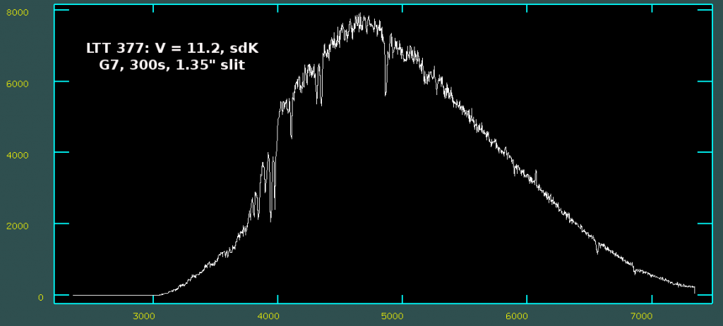
| a0053955_1D | G4 | 4.1 | LTT_377 | 600 | 2.1″ slit in 1.5″ seeing |
| a0071045_1D | G7 | 17.0 | LTT_377 | 300 | 1.35″ slit in ? seeing |
| a0071110_1D | G7 | 15.3 | EG21 | 300 | 2.1″ slit in 1.2″ seeing |
A more detailed version of this table: NOTES
The observed S/N may be simply estimated in the wavelength range of interest by, for example in python:
x,y = np.loadtxt(‘a0071110_1D.txt’,unpack=True, usecols=(0,1)) # read in data
ok = np.where( (x>5100.) & (x<5200.) )[0] # choose wavelength range relatively free of absorption lines
print median(y[ok])/std(y[ok])
76.043849269
Therefore, for LTT 377 at ~5150A (flux ~1.2e-13 erg/s/cm^2/A) SpUpNIC reaches a S/N ~76 PER CCD PIXEL in 600s.
Flux calibration curves
gr7_calfac_grang17.0
gr7_calfac_grang15.3
gr4_calfac_grang4.1
The Hamuy standards used in the calibration can be found here:
ftp://ftp.eso.org/pub/stecf/standards/ctiostan/ NOTE: LTT377 is cd_34d241
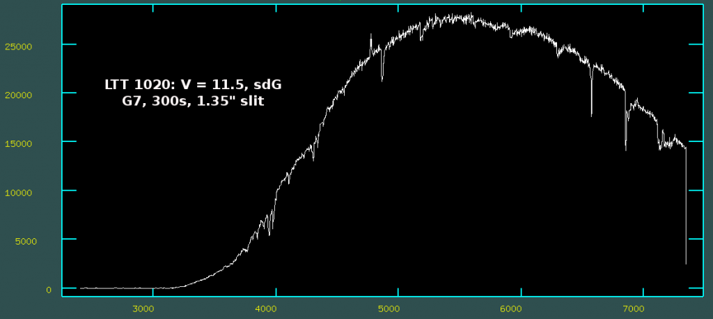
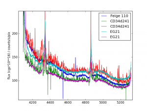
Approximate polynomial fits to a series of standard stars, giving the factor by which to multiply the raw counts (per second), to get to flux, as described above. The plots below show the stars used (and the variation from object-to-object) for G4 and G7 respectively. Note: LTT1020 seems to be an outlier and has been rejected from the fits. It may be necessary to interpolate the wavelengths onto a common grid before multiplying.

Quick Python Example:
x,y = np.loadtxt(‘a0071110_1D.txt’,unpack=True, usecols=(0,1)) # read in data
y = y / 600. # convert to counts/s
a,b = np.loadtxt(‘gr7_calfac_grang15.3.txt’,unpack=True, usecols=(0,1)) # read in appropriate flux conversion factor
# interpolate to same wavelength bins:
ib = np.interpol(x,a,b)
plot(x, y*ib*1e-16 ) # flux calibrated in erg/s/cm^2/A
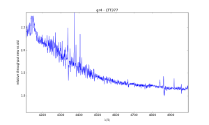
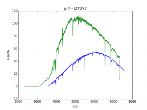
Comparison with Pre-Upgrade Spectrograph
For users preferring to scale their exposure times from previous experience, the following may be more useful.
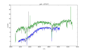
G4
Comparison of pre-upgrade (blue) vs SpUpNIC (green) in e-s per second **per A**. Note: the dispersion has changed from 0.495 A/pix to 0.622 A/pix and this conversion factor has been included. The old gain was 1e-/ADU. To compare values per CCD pixel, SpUpNIC will be 0.622/0.495 times higher than plotted. To compare old and new counts, SpUpNIC will be 1.145 times lower (the new gain).
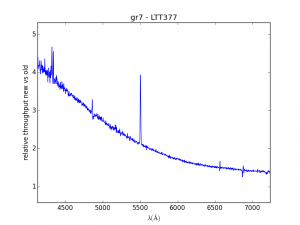
Relative throughput (ratio of the above). Not smoothed.
As above, but for G7.
SpUpNIC Instrument Team
SpUpNIC was an effort undertaken by a large team of people, over a very long period of time. The PI on the project was Lisa Crause (aka the fearless leader).
We encourage proper credit be given to the instrument teams, which means that co-authorship for the following groups would be appreciated for publications stemming from data taken during commissioning time. This follows the standard instrument commissioning agreement for SpUpNIC.
Full Instrument Team
L.A. Crause, D.B. Carter, A. Daniels, G.P. Evans, P. Fourie, D. G. Gilbank, M. Hendricks, W. Koorts, D. Lategan, E. Loubser, S. Mouries, J. O’Connor, D. O’Donoghue, S.B. Potter, C. Sass, A.A. Sickafoose, J. Stoffels, P. Swanevelder, C. van Gend, M. Visser, H.L. Worters
The full team includes all staff who have made a significant contribution to the project. Notably, this includes workshop staff and technicians (non-scientists).
Typically, the instrument PI is the lead author on the papers and publications in which the instrument is described. Regardless of the first author, the full instrumentation team should be provided the opportunity to be coauthors on the first instrument presentation (e.g. at an SPIE meeting) and on the instrument publication. The decision to be a co-author rests with each individual, such that they can opt out if desired.
Instrument Science Team
L.A. Crause, D. G. Gilbank, D. O’Donoghue, S.B. Potter, A.A. Sickafoose, C. van Gend, H.L. Worters
The science team consists of PhD-level staff who have contributed significant time and/or effort to the construction of the instrument. This is a subset of the full instrument team.
Users of an instrument while it is undergoing commissioning are strongly encouraged to credit the instrument science team in all publications stemming from data taken during that time. Without these people, the instrument would not be available!
HIPPO: High speed Photo-Polarimeter
HIPPO is SAAO’s newest (2008) high-speed photo-polarimeter. It is capable of high-speed, multi-filtered, simultaneous all-Stokes observations of point sources. Its high-speed capabilities make it especially ideal for investigating rapidly varying astronomical sources such as magnetic cataclysmic variables. HIPPO was designed and built in order to replace its highly successful but ageing single channel equivalent, namely the University of Cape Town (UCT) photo-polarimeter (Cropper 1985).
The instrument makes use of rapidly counter-rotating (10Hz), super-achromatic half- and quarter-waveplates, a fixed Glan-Thompson beamsplitter and two photo-multiplier tubes that record the modulated O and E beams. Each modulated beam permits an independent measurement of the polarisation and therefore simultaneous 2 filter observations. All Stokes parameters are recorded every 0.1sec and photometry every 1 millisecond. Post-binning of data is possible in order to improve the signal. First light was obtained in February 2008.
Current Status & Availability
HIPPO is open for general use on the 1.9m telescope only. Potential applicants should contact the PI (Stephen Potter: sbp at saao dot ac dot za) if first time users or would like to collaborate.
The HIPPO control software runs on a Linux operating system with a real-time linux kernel patch in order to guarantee absolute and relative timing accuracies. On-the-fly preliminary data reduction produces live photometry and polarimetry light curves.
A user manual is available here and a reference manual is available here.
Offline Data Reduction
A set of data reduction algorithms are available. The routines are written for unix based operating systems (Linux and MacOS) and are compiled (e.g. using a gcc compiler) and executed from the command line. The data reduction process in split into three sets of reduction routines written in C. The first set deal with splitting the raw data file(s) into more manageable files sorted by target name, filter and channel. The second set extracts the photometry and handles binning, sky-subtraction and co-adding. The third set extracts the polarisation and handles binning, sky-subtraction, co-adding and polarisation calculation.
Software and sample reduction instructions are currently available upon request (Stephen Potter: sbp at saao dot ac dot za).
Publications
Please email the PI (Stephen Potter: sbp at saao dot ac dot za) if you are aware of any publications that have made use of HIPPO observations that are not listed below.
Yudin, R. V.; Potter, S. B.; Townsend, L. J. 2017MNRAS.464.4325, First multicolour polarimetry of TeV γ-ray binary HESS J0632+057 close to periastron passage
Buckley, D. A. H.; Meintjes, P. J.; Potter, S. B.; Marsh, T. R.; Gänsicke, B. T. 2017NatAs…1E..2, Polarimetric evidence of a white dwarf pulsar in the binary system AR Scorpii
Pekeur, N. W.; Taylor, A. R.; Potter, S. B.; Kraan-Korteweg, R. C., 2016MNRAS.462L..80 Evidence for quasi-periodic oscillations in the optical polarization of the blazar PKS 2155-304
Potter, Stephen B., 2016ASSL..439..179 Stokes Imaging: Mapping the Accretion Region(s) in Magnetic Cataclysmic Variables
Potter, S.B. 2015AcPPP…2..139 High-Speed Photo-Polarimetry of Magnetic Cataclysmic Variables
Buckley, D. A. H.; Potter, S. B.; Kotze, E.; Kotze, M.; Breytenbach, H. 2014EPJWC..6407005 New Observations of Accretion Phenomena in Magnetic Cataclysmic Variables
Kniazev A. Y. et al. ApJ, 2013, 770, 124: Characterization of the nearby L/T Binary Brown Dwarf WISE J104915.57-531906.1 at 2 Pc from the Sun
Potter S. The fourth Gaia Science Alerts workshop, 2013: South African Astronomy and Observatories
Potter S. IAUS, 2012, 285, 117: Polarimetric Variability
Potter et al, MNRAS, 2012, 420, 2596: On the spin modulated circular polarization from the intermediate polars NY Lup and IGR J15094-6649
Potter S., LSST all hands meeting, 2012: Time Domain Science and LSST Follow-up in South Africa
Andersson B.-G.; Potter S. B. ASPC, 2011, 449, 134: Observational Evidence for Radiative Interstellar Grain Alignment
Potter S. et al, ASPC, 2011, 449, 27: First Science Results from the High Speed SAAO Photo-polarimeter
Potter S. et al, MNRAS, 2011, 416, 2202: Possible detection of two giant extrasolar planets orbiting the eclipsing polar UZ Fornacis
Revnivtsev M. et al. MNRAS, 2011, 411, 1317: Observational evidence for matter propagation in accretion flows
Russell D. et al. 2011,ArXiv1104, 837: Rapid variations of polarization in low-mass X-ray binaries
Russell D. et al. PoS, htra-IV, 2010: Rapid variations of polarization in low-mass X-ray binaries
Andersson B.-G.; Potter S. B. ApJ, 2010, 720, 1054: Observations of Enhanced Radiative Grain Alignment Near HD 97300
Andersson B.-G.; Potter S. B. AAS, 2010, 42, 320: Observations of Enhanced Radiative Grain Alignment Near HD 97300
Potter S. et al. MNRAS, 2010, 402, 1161: Polarized QPOs from the INTEGRAL polar IGRJ14536-5522 (=Swift J1453.4-5524) also describes HIPPO commissioning
Potter S. et al. SPIE, 2008, 7014, 179: A new two channel high-speed photo-polarimeter (HIPPO) for the SAAO
SHOC: Sutherland High Speed Optical Cameras
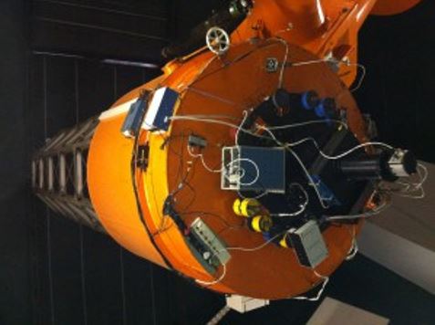
SHOC: Sutherland High Speed Optical Cameras
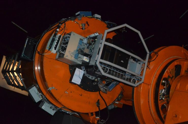
SHOC mounted with the focal reducer on the 1.9m telescope. The large bluish rectangle near the center of the image is the box containing the SHOC computer and electronics; the camera is the small gray object at the end of the long, black focal reducer tube.
Two nearly identical instruments named SHOC are available for use on the SAAO 1.9-m and 1.0-m telescopes, and on the new 1.0-m telescope, Lesedi. SHOC 1 and 2 are high-speed, visible-wavelength systems, mounted at Cassegrain focus and using the existing filter wheels employed by the SAAO CCDs. The SHOC cameras allowed the UCT CCD camera to be decommissioned in 2012.
The SHOC design is based on POETS (Portable Occultation, Eclipse, and Transit Systems; developed by a collaboration between groups at the Massachusetts Institute of Technology (MIT) and Williams College) and MORIS (MIT Optical Rapid Imaging System) at NASA’s 3-m IRTF on Mauna Kea, Hawaii.
Technical Specifications
The SHOC instruments employ Andor iXon 888 EM CCD cameras, which have an electron-multiplying (EM) capability. They are 2048×1024 13-μm pixel detectors, operated in frame-transfer mode (imaging area 1024×1024 pixels). The following characteristics apply:
| Telescope | Field of View (arcmin) | Instrument | Platescale (arcsec/pixel) |
| 1.9m | 1.29 x 1.29 | Spectrograph, CCD cameras | 0.076 |
| 1.9m + focal reducer | 2.79 x 2.79 | Spectrographs, CCD Cameras, Polarimeter | 0.163 |
| 1.0m | 2.85 x 2.85 | CCD cameras | 0.167 |
| Lesedi | 5.72 x 5.72 | CCD cameras, spectrograph coming soon | 0.335 |
The cameras have selection of amplifiers (four different speeds; two conventional and four EM), each having multiple electron to ADU gain settings. Binning and subframing are also user selectable. Operating at the lowest readout speed (lowest read noise) with appropriate binning for Sutherland’s median seeing, a minimum cycle time of ~0.5 seconds is typical. With further binning, windowing and higher readout speed, the cycle time can be decreased to 0.01 seconds. The SHOC 1 and 2 systems contain identical components, except that the cameras have slightly different technical properties (read noise, well depth, etc.). See the SHOC 1 camera specification sheet and the SHOC 2 camera specification sheet.
There is an online calculator to help with estimating observing times, signal-to-noise ratios, and limiting magnitudes.
Current Status & Availability
The instruments are open for general use. The software has been overhauled and integrated during the two years following commissioning, and is now running on a web-based platform with js9 display. Please note the following:
- Use of EM mode is prohibited unless demonstrated competence of this mode is provided, due to the risk of permanent damage to the CCD. Future software will incorporate safeguards to protect the detector in EM mode. In the meantime, observing in EM mode is highly regulated.
- External start mode with the 3 MHz amplifier is not currently available on SHOC 2. Please instead use External timing, a different amplifier, or specifically request SHOC 1.
Observers are invited to apply for time using SHOC on the 1.9-m and 1.0-m telescopes. SHOC 2 is currently mounted on the new 1.0-m telescope at all times. Those new to SHOC must request assistance for the first night of their run; students must be accompanied by their supervisor. Please reference the SHOC instrument paper in your publications (see below).
Filters
Lesedi has its own filter wheel containing Bessell U B V R I and clear filters. Only these filters are available on this telescope at the present time.
For the 1.9-m and original 1.0-m telescopes, the available filter sets are listed below (click on filter name to view transmission curve); there is also an empty slot in each filter wheel for white light observations:
- Bessell U B V R I
- SDSS u’ g’ r’ i’ z’
- Hα wide (20 nm)
- Hα narrow (3 nm)
- Redshifted Hα at 667, 681 & 686 nm
- [O III] 501 nm
- BG38
- Z
Please be sure to list every filter you require for your program in the GRATINGS AND FILTERS field of the SAAO Telescope Time Application form. This will ensure that your desired filters are scheduled for your run.
Visitor filters up to 51 mm square and 10 mm thick can also be accommodated. Visitors wishing to use their own filters should contact the Head of Telescope Operations (rrs at saao.ac.za) to discuss this when applying for telescope time.
Further Information
Further information can be found on the SHOC commissioning website. Available here are links to the online user manual and the SHOC data reduction pipeline (start with the README!).
Selected publications from commissioning:
- SHOC instrument paper: Coppejans, R. et al., 2013, Characterizing and Commissioning the Sutherland High-Speed Optical Cameras (SHOC), PASP, 125, 976-988
- P. Woudt, et. al., 2012, CC Sculptoris: a superhumping intermediate polar, MNRAS, 427, 1004-1013
- D. Coppejans, et al. 2013, High-speed photometry of faint cataclysmic variables -VIII. Targets from the Catalina Real-time Transient Survey, MNRAS, 437, 510-523
- A.N. Semena, et al., 2014, On the area of accretion curtains from fast aperiodic time variability of intermediate polar EX Hya, MNRAS, 442, 1123-1132.
- D. de Martino et al., 2014, Unveiling the redback nature of the low-mass X-ray binary XSS J1227.0-4859 through optical observations, MNRAS, 444, 3004-3014.
SAAO CCD Camera (STE3/STE4)
Two SAAO CCD cameras are available for direct imaging on the 1.0-m telescope, but currently unavailable on the 1.9-m telescope due to failure of the DOS control system. The two cameras are distinguished by their detectors: STE4, a 1024×1024 pixel back-illuminated CCD, and STE3, a 512×512 pixel version of the same chip, with one quarter of the field of view of STE4. The control software is Linux-based (manual available here). Software is available at the telescope for determining guide star positions, as described in the TCS manual for each telescope.
Filters
Bessell U B V R I filters are available for use with the SAAO CCDs and are mounted at all times (click on filter name to view transmission curve); there is also an empty slot in the filter wheel for white light observations. We have one of each of the following filters, available on request:
Please be sure to list every filter you require for your program in Section 4 of the SAAO Telescope Time Application form. This will ensure that your desired filters are scheduled for your run.
Visitor filters up to 51 mm square and 10 mm thick can also be accommodated. Visitors wishing to use their own filters should contact the Head of Telescope Operations (rrs at saao.ac.za) to discuss this when applying for telescope time.
Detector Properties
The table below gives the properties of STE4. Where the attributes of STE3 differ, they are given in square brackets.
| DEVICE NAME | STE4 [STE3] |
| Manufacturer | SITe |
| Chip Type | Back-illuminated |
| Number of Pixels | 1024×1024 [512×512] |
| Pixel size | 24 microns square |
| Scale (1.0-m) | 0.31 arcsec/pix |
| Scale (1.9-m) | 0.14 arcsec/pix |
| Field of view (1.0-m) | 317″x317″ [158″x158″] |
| Field of view (1.9-m) | 146″x146″ [73″x73″] |
| Read Noise | 6.5 e– [5 e–] |
| Scale Factor | 2.8 e–/ADU [1.9 e–/ADU] |
| Linear Count Limit | 65535 ADU |
| Readout Time (unbinned) | 43 sec [17 sec] |
| Prebin options | 1×1, 2×2 |
| U zero point (1ADU/sec)(STE4 on 1.0-m) | 19.20 mag |
| B | 22.00 mag |
| V | 22.35 mag |
| I | 21.80 mag |
Data Reduction
There are Linux PCs located in the domes for image processing using IRAF and a pipeline based on DoPHOT. The latter can be used for real-time reductions, to obtain reduced CCD photometry of stellar fields while observing. As each image is written to disc, the program picks out the correct flatfield, cleans and flatfields the frame and writes it out as a FITS file. It then runs DoPHOT on the image to produce aperture and profile-fitted magnitudes. If you are observing the same field repeatedly, DoPHOT will display differential profile-fitted magnitudes as a function of time. The results from DoPHOT can be further processed using routines in the local STAR package to produce the final results.
Data Backup & Archiving
Observers can backup their data to their laptop, or transfer it to their home institute via ftp. Alternatively, observers may arrange with IT staff to write their data to DVD for them. The computers in the domes do not have DVD-writing facilities, nor functioning USB ports.
Sibonise
Sibonise, meaning “show us” in isiXhosa, is currently being commissioned on Lesedi. It is an imaging camera with the largest detector of any SAAO instrument, an E2V 6kx6k pixel CCD, yielding a field of view of two thirds of a degree in diameter. A summary of the key features can be found in the table below, with more details to follow shortly.
| Detector | E2V CCD231-C6 back-illuminated, NIMO |
| No. of pixels | 6144×6160 |
| Field of view | 39 arcmin diameter |
| Platescale | 0.77 acrsec/pixel |
| Coating | Astro multi-2 |
| Filters | U, B, V, R, I, Hα, [O III], clear |
—